Objectives¶

• Compare reads to assemblies
• Compare datasets and build a clustermap

K-mers!¶

K-mers are a fairly simple concept that turn out to be tremendously powerful.

A “k-mer” is a word of DNA that is k long:

ATTG - a 4-mer
ATGGAC - a 6-mer

Typically we extract k-mers from genomic assemblies or read data sets by running a k-length window across all of the reads and sequences – e.g. given a sequence of length 16, you could extract 11 k-mers of length six from it like so:

AGGATGAGACAGATAG

becomes the following set of 6-mers:

AGGATG
 GGATGA
  GATGAG
   ATGAGA
    TGAGAC
     GAGACA
      AGACAG
       GACAGA
        ACAGAT
         CAGATA
          AGATAG

k-mers are most useful when they’re long, because then they’re specific. That is, if you have a 31-mer taken from a human genome, it’s pretty unlikely that another genome has that exact 31-mer in it. (You can calculate the probability if you assume genomes are random: there are 4³¹ possible 31-mers, and 4³¹ = 4,611,686,018,427,387,904. So, you know, a lot.)

The important concept here is that long k-mers are species specific. We’ll go into a bit more detail later.

K-mers and assembly graphs¶

We’ve already run into k-mers before, as it turns out - when we were doing genome assembly. One of the three major ways that genome assembly works is by taking reads, breaking them into k-mers, and then “walking” from one k-mer to the next to bridge between reads. To see how this works, let’s take the 16-base sequence above, and add another overlapping sequence:

AGGATGAGACAGATAG
    TGAGACAGATAGGATTGC

One way to assemble these together is to break them down into k-mers –

becomes the following set of 6-mers:

AGGATG
 GGATGA
  GATGAG
   ATGAGA
    TGAGAC
     GAGACA
      AGACAG
       GACAGA
        ACAGAT
         CAGATA
          AGATAG -> off the end of the first sequence
           GATAGG <- beginning of the second sequence
            ATAGGA
             TAGGAT
              AGGATT
               GGATTG
                GATTGC

and if you walk from one 6-mer to the next based on 5-mer overlap, you get the assembled sequence:

AGGATGAGACAGATAGGATTGC

Graphs of many k-mers together are called De Bruijn graphs, and assemblers like MEGAHIT and SOAPdenovo are De Bruijn graph assemblers - they use k-mers underneath.

Why k-mers, though? Why not just work with the full read sequences?¶

Computers love k-mers because there’s no ambiguity in matching them. You either have an exact match, or you don’t. And computers love that sort of thing!

Basically, it’s really easy for a computer to tell if two reads share a k-mer, and it’s pretty easy for a computer to store all the k-mers that it sees in a pile of reads or in a genome.

Long k-mers are species specific¶

So, we’ve said long k-mers (say, k=31 or longer) are pretty species specific. Is that really true?

Yes! Check out this figure from the MetaPalette paper:

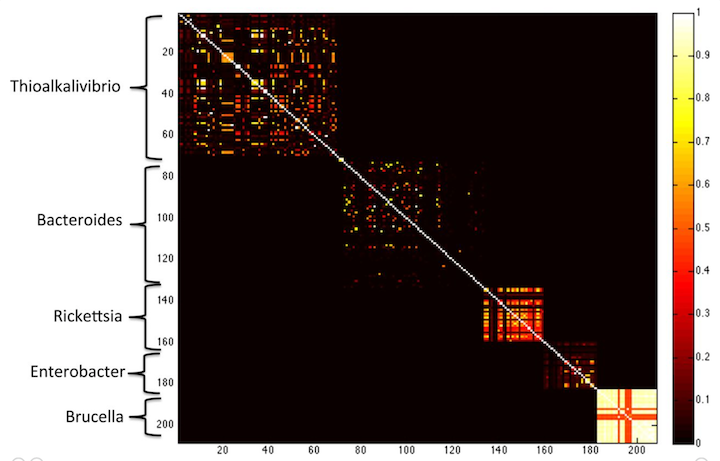
here, the Koslicki and Falush show that k-mer similarity works to group microbes by genus, at k=40. If you go longer (say k=50) then you get only very little similarity between different species.

Using k-mers to compare samples against each other¶

So, one thing you can do is use k-mers to compare genomes to genomes, or read data sets to read data sets: data sets that have a lot of similarity probably are similar or even the same genome.

One metric you can use for this comparisons is the Jaccard distance, which is calculated by asking how many k-mers are shared between two samples vs how many k-mers in total are in the combined samples.

only k-mers in both samples
----------------------------
all k-mers in either or both samples

A Jaccard distance of 1 means the samples are identical; a Jaccard distance of 0 means the samples are completely different.

This is a great measure and it can be used to search databases and cluster unknown genomes and all sorts of other things! The only real problem with it is that there are a lot of k-mers in a genome – a 5 Mbp genome (like E. coli) has 5 m k-mers!

About a year ago, Ondov et al. (2016) showed that MinHash approaches could be used to estimate Jaccard distance using only a small fraction (1 in 10,000 or so) of all the k-mers.

The basic idea behind MinHash is that you pick a small subset of k-mers to look at, and you use those as a proxy for all the k-mers. The trick is that you pick the k-mers randomly but consistently: so if a chosen k-mer is present in two data sets of interest, it will be picked in both. This is done using a clever trick that we can try to explain to you in class - but either way, trust us, it works!

We have implemented a MinHash approach in our sourmash software, which can do some nice things with samples. We’ll show you some of these things next!

Installing sourmash¶

To install sourmash, run:

sudo apt-get -y update && \
sudo apt-get install -y python3.5-dev python3.5-venv make \
    libc6-dev g++ zlib1g-dev

this installs Python 3.5.

Now, create a local software install and populate it with Jupyter and other dependencies:

python3.5 -m venv ~/py3
. ~/py3/bin/activate
pip install -U pip
pip install -U Cython
pip install -U jupyter jupyter_client ipython pandas matplotlib scipy scikit-learn khmer

pip install -U https://github.com/dib-lab/sourmash/archive/master.zip

Generate a signature for Illumina reads¶

Download some reads and the assembled metagenome:

mkdir ~/work
cd ~/work
curl -L -o SRR1976948.abundtrim.subset.pe.fq.gz https://osf.io/k3sq7/download
curl -L -o SRR1976948.megahit.abundtrim.subset.pe.assembly.fa https://osf.io/dxme4/download
curl -L -o SRR1976948.spades.abundtrim.subset.pe.assembly.fa https://osf.io/zmekx/download

Compute a scaled MinHash signature from our reads:

mkdir ~/sourmash
cd ~/sourmash

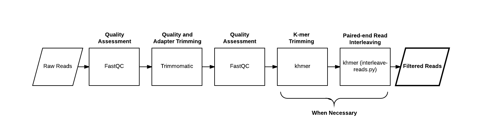
First let’s compute a signature for some reads from the Hu et al., 2016 <http://mbio.asm.org/content/7/1/e01669-15.full>__. paper. These reads have been both quality trimmed and k-mer trimmed. In practice it may be important to compare outcomes with and without k-mer trimming.

sourmash compute -k51 --scaled 10000 ../work/SRR1976948.abundtrim.subset.pe.fq.gz -o SRR1976948.reads.scaled10k.k51.sig 

Compare reads to assemblies¶

Use case: how much of the read content is contained in our assembled metagenome?

Build a signature for an assembled metagenome:

sourmash compute -k51 --scaled 10000 ../work/SRR1976948.spades.abundtrim.subset.pe.assembly.fa -o SRR1976948.spades.scaled10k.k51.sig 
sourmash compute -k51 --scaled 10000 ../work/SRR1976948.megahit.abundtrim.subset.pe.assembly.fa -o SRR1976948.megahit.scaled10k.k51.sig

and now evaluate containment, that is, what fraction of the read content is contained in the genome:

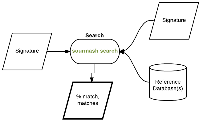
sourmash search SRR1976948.reads.scaled10k.k51.sig SRR1976948.megahit.scaled10k.k51.sig --containment 
sourmash search SRR1976948.reads.scaled10k.k51.sig SRR1976948.spades.scaled10k.k51.sig --containment

You should see something like:

loaded query: SRR1976948.abundtrim.subset.pe... (k=51, DNA)
loaded 1 signatures and 0 databases total.                                     
1 matches:
similarity   match
----------   -----
 48.7%       SRR1976948.megahit.abundtrim.subset.pe.assembly.fa

loaded query: SRR1976948.abundtrim.subset.pe... (k=51, DNA)
loaded 1 signatures and 0 databases total.                                     
1 matches:
similarity   match
----------   -----
 47.5%       SRR1976948.spades.abundtrim.subset.pe.assembly.fa

Why are only ~40% of our reads in the genome?

Try the reverse - why is it bigger?

sourmash search SRR1976948.megahit.scaled10k.k51.sig SRR1976948.reads.scaled10k.k51.sig --containment
sourmash search SRR1976948.spades.scaled10k.k51.sig SRR1976948.reads.scaled10k.k51.sig  --containment

loaded query: SRR1976948.megahit.abundtrim.s... (k=51, DNA)
loaded 1 signatures and 0 databases total.                                     
1 matches:
similarity   match
----------   -----
 99.8%       SRR1976948.abundtrim.subset.pe.fq.gz

loaded query: SRR1976948.spades.abundtrim.su... (k=51, DNA)
loaded 1 signatures and 0 databases total.                                     
1 matches:
similarity   match
----------   -----
 99.9%       SRR1976948.abundtrim.subset.pe.fq.gz

(...but ~ 99% of our k-mers from the genome are in the reads!?)

This is basically because of sequencing error! Illumina data contains a lot of errors, and the assembler doesn’t include them in the assembly!

Compare signatures.¶

First, to make our comparison more interesting let’s grab some signatures for the other datasets and assemblies for this study.

Instead of running curl a bunch of times, we can use osfclient to download a bunch of files by name:

pip install osfclient

osf -p ay94c fetch osfstorage/signatures/SRR1977249.megahit.scaled10k.k51.sig SRR1977249.megahit.scaled10k.k51.sig
osf -p ay94c fetch osfstorage/signatures/SRR1977249.reads.scaled10k.k51.sig SRR1977249.reads.scaled10k.k51.sig
osf -p ay94c fetch osfstorage/signatures/SRR1977249.spades.scaled10k.k51.sig SRR1977249.spades.scaled10k.k51.sig
osf -p ay94c fetch osfstorage/signatures/SRR1977296.megahit.scaled10k.k51.sig SRR1977296.megahit.scaled10k.k51.sig
osf -p ay94c fetch osfstorage/signatures/SRR1977296.reads.scaled10k.k51.sig SRR1977296.reads.scaled10k.k51.sig
osf -p ay94c fetch osfstorage/signatures/SRR1977296.spades.scaled10k.k51.sig SRR1977296.spades.scaled10k.k51.sig
osf -p ay94c fetch osfstorage/signatures/subset_assembly.megahit.scaled10k.k51.sig subset_assembly.megahit.scaled10k.k51.sig

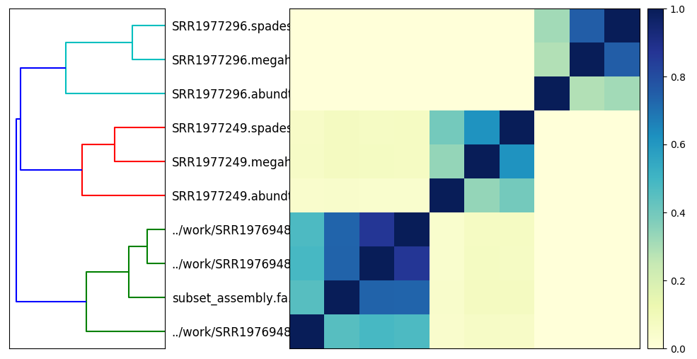
Now, let’s compare these signatures and plot their jaccard similarities

Compare all the signatures:

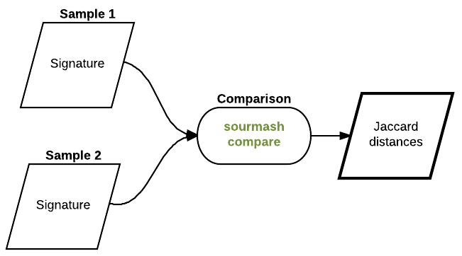
sourmash compare *sig -o Hu_metagenomes

and then plot:

sourmash plot --labels Hu_metagenomes

which will produce a file Hu_metagenomes.dendro.png and Hu_metagenomes.matrix.png which you can then download via FileZilla and view on your local computer.

Now open jupyter notebook and visualize:

from IPython.display import Image
Image("Hu_metagenomes.matrix.png")

Here’s a PNG version:

What can we do now?

• More k-mer exploration
• Taxonomic classfication
• Functional analysis